Antares is the morning star of the summer sky. Rising at the head of the Scorpion an hour before the southern Milky Way, it heralds the arrival the most brilliant season in the celestial year — a season which, despite its short nights and bothersome bugs, is packed full with unique deep-sky objects, in addition to the Milky Way which never gets old. The summer sky objects are my favorites, and Antares is the best of them all.
P.S. Happy Canada Day! Today’s subject is too far south to be imaged clearly from Canada 😛
1. Zoomed Out (24mm pano, Potter Valley)
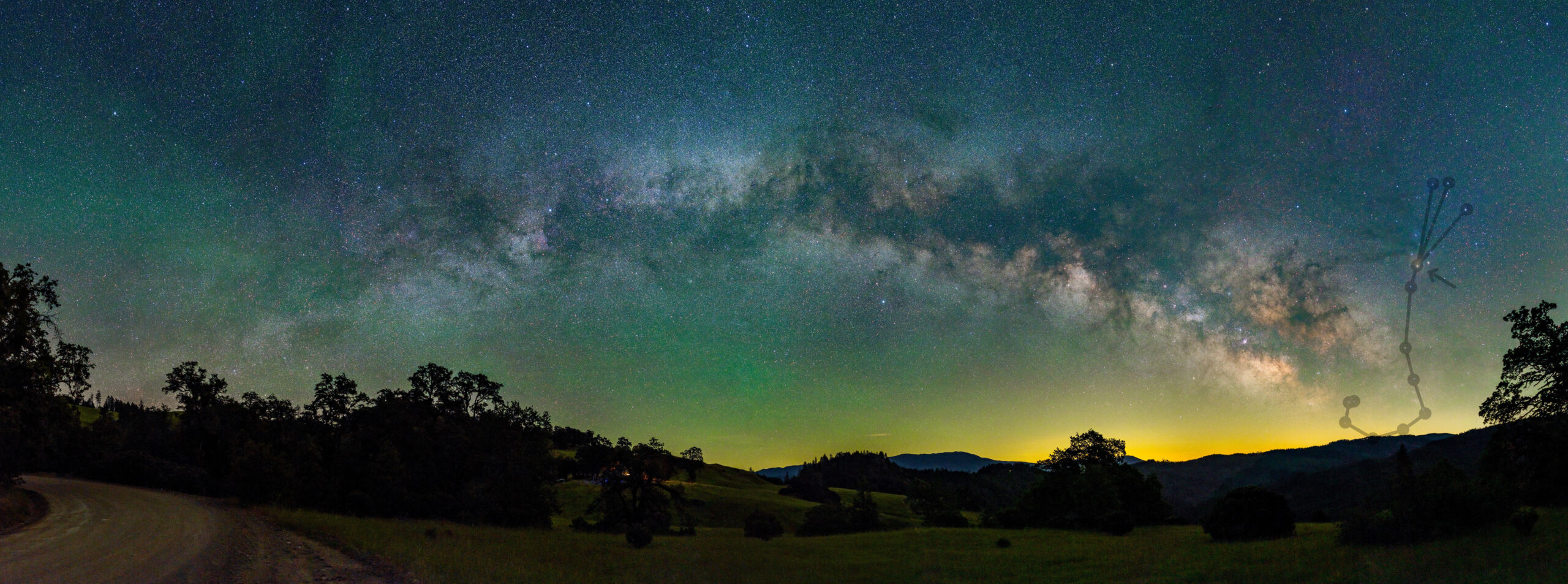
Let’s set the stage by locating Antares in the night sky. Below is a panorama of the rising Milky Way, taken from a remote country road off CA-20, some 2 hours north of San Francisco. We are facing east, and I have highlighted the constellation Scorpius in the right of the photo, to the south. Antares is the bright yellow star at the scorpion’s mouth.
Below, I give a slightly zoomed-in view, taken an hour later a mile down the road. This photo shows finer detail, since it is a mosaic of shots taken from a longer focal-length lens (Sony 50mm GM vs. Sigma 24mm DN Art). I won’t point to Antares here, but if you were paying attention, it should be easy to find! Looking closely, you should see black “dust clouds” emanating from the star, like smoke from a campfire blowing in the wind. Look still closer and you can see a faint blue glow in one of the stars above (that’s Rho Ophiuchi) and a large but fainter glow to the upper-right (Blue Horsehead Nebula). There is also what looks like a diffuse “white star” to the right of Antares — that’s the Crab Globular Cluster (M4), a group of hundreds of thousands of stars over 6,000 light-years away. And the attentive eye will notice a faint red glow to the right around the star Alniyat.
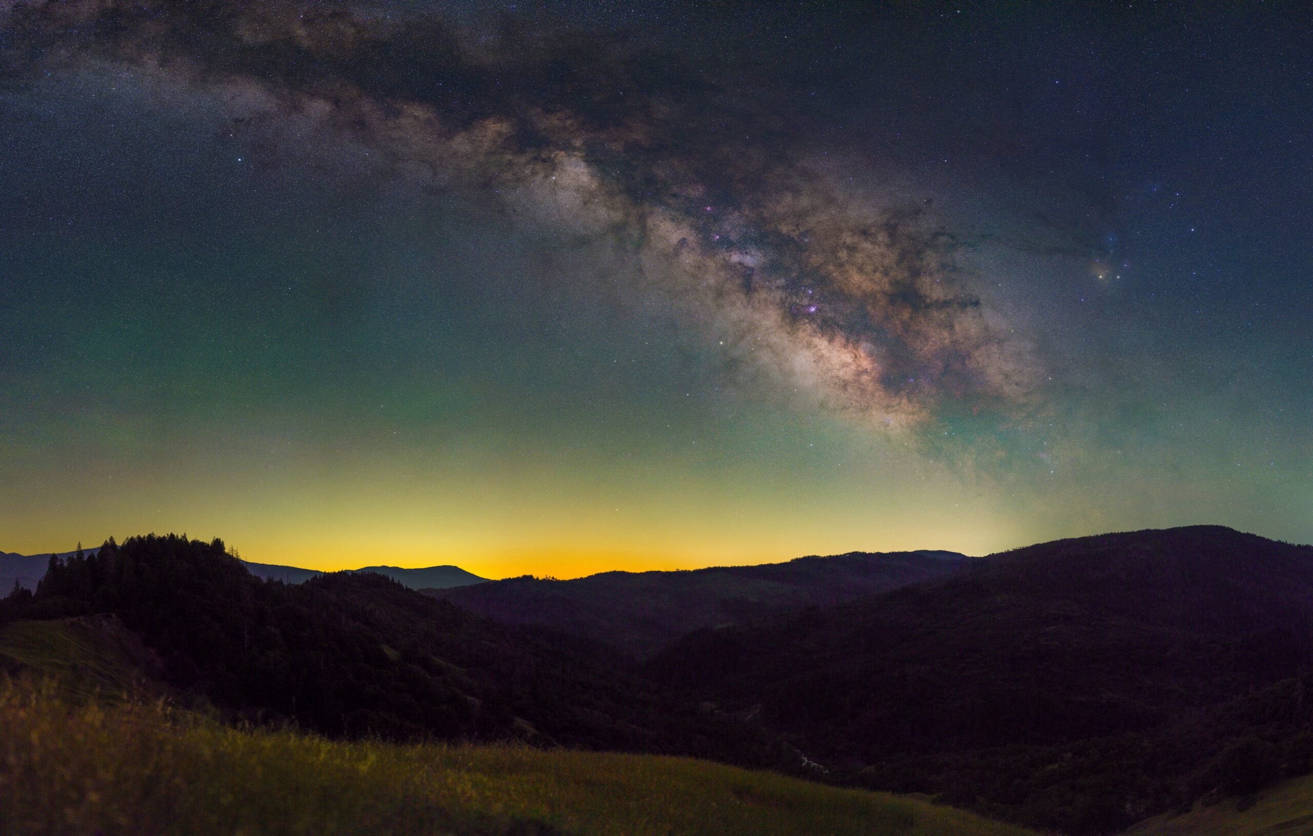
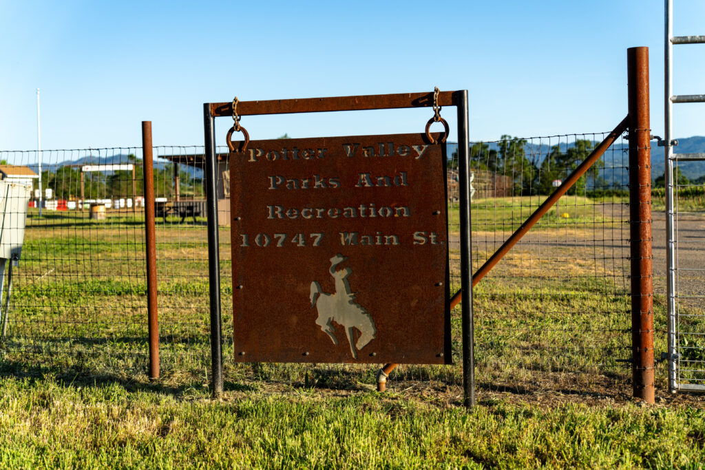
Any dark-sky site with a clear view south will see Antares in early summer. These photos were taken during a weekend outing at Potter Valley, a farming town outside Ukiah, where I originally went to catch the northern Milky Way. The north horizon was blocked by hills from this vantage point. The south view was unobstructed over the scenic river valley, but you can still see the strong glow of light pollution from the many small settlements to the southeast.
2. Neighborhood of Antares (85mm, Big Sur)
Potter Valley has a horse race grounds and they were setting up for the annual rodeo that month. But this was not my first rodeo. Two weeks earlier, I had been down to Big Sur to try out 50mm panoramas for the first time. It was a very clear night and you could even see the moon set, without any clouds in the way:
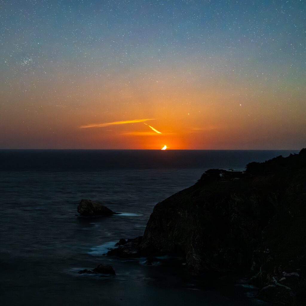
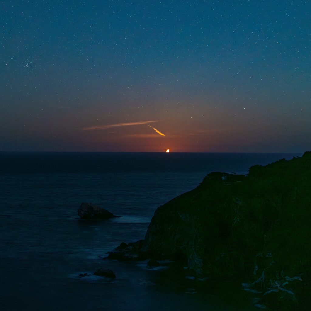
After the moonset, while I was waiting for the galactic core to rise, I took out my 85mm Sigma Art (bought in Japan, see this post), placed the camera on a cheap Teseek star tracker (from Aliexpress), and collected 20 minutes of frames. This was difficult owing to the winds, which get amplified by the Big Sur topography. But I got enough frames to construct a decent image. Here’s an example of a single 10-second frame:
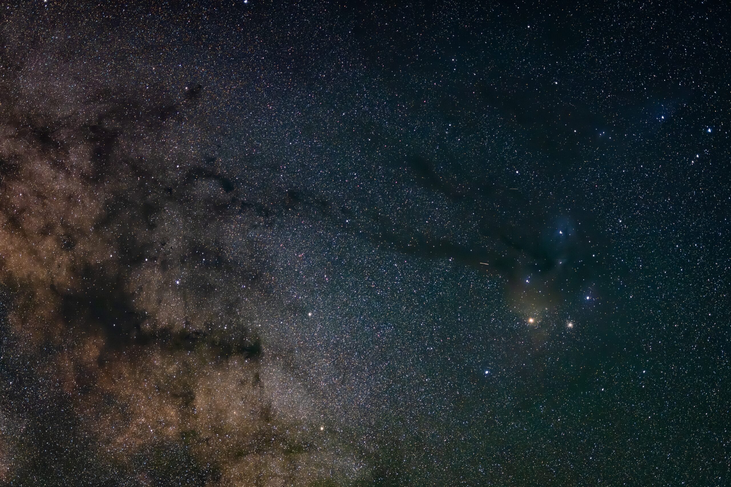
And here’s the final image:
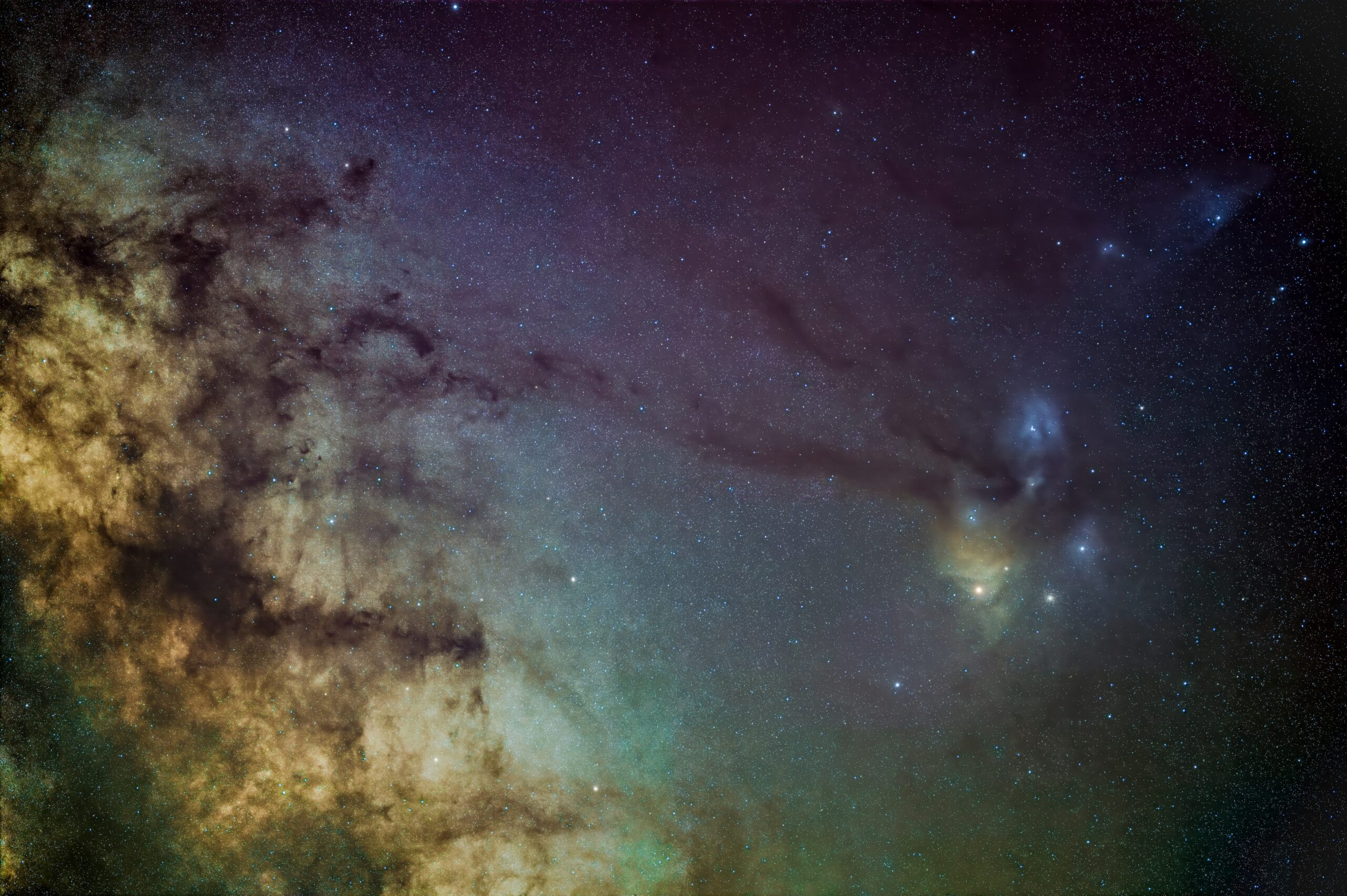
This carries much more detail than the panorama. The blue nebulae stand out prominently! And you can clearly see that M4 is a star cluster, not a single star. But there are a few things that I dislike about this photo:
- There were colorful background gradients that were difficult to subtract. For wide-field, gradients are great: they create the frame that adds character to a starscape. This includes green airglow, the golden dawn of the moonrise, and (to an extent) those yellow light domes over cities. But deep-sky photos are too zoomed-in to appreciate this background, which becomes a “haze” that prevents you from resolving the full contrast of the target image. That’s what’s happening here. And gradients are most prominent along the horizon. If I had shot this further south (say Baja California), I would have obtained a much cleaner image.
- The Sony camera filters out most of the H-alpha emission around the star Alnitak (see discussion on this post). In a full-spectrum camera, that region would light up a bright red, adding a pleasing contrast to the yellows, blues, and grays.
Maybe in the future, when I get the chance to visit Baja California or Taiwan or any other low-latitude destination, I will try this shot again. Antares climbs much higher in the sky from those spots, so I could avoid the gradients. Combining this with an astro-modified camera on a star tracker (still portable in carry-on!), I could get a really pleasing image at this focal length.
3. Zoomed in — too far! (530mm, Baxter Park)
The third view of Antares is one that I’ve already discussed. A year ago, I visited Baxter State Park and shot the nebula with the 530mm Takahashi FSQ-106N. The resulting image was incredibly detailed, but a little too far zoomed-in to see all the objects. I can frame Antares, the Crab cluster, Alnitak, and some of the surrounding H-alpha. But I’m missing that bright blue Rho Ophiuchi nebula — cut off at the top.
4. Just right! (250mm, Pigeon Point / Williams)
Traveling for work in California again, June gloom had set in and there was not much clear sky. Early summer wind patterns bring in cool ocean air as the inland country heats up. This makes mornings cloudy, and while the clouds evaporate by mid-day, the breeze does not stop, and evenings are cloudy too. This gives pleasant temperatures, but not-so-pleasant astronomy. Fortunately, there were a couple of nights around the new moon when the clouds broke.
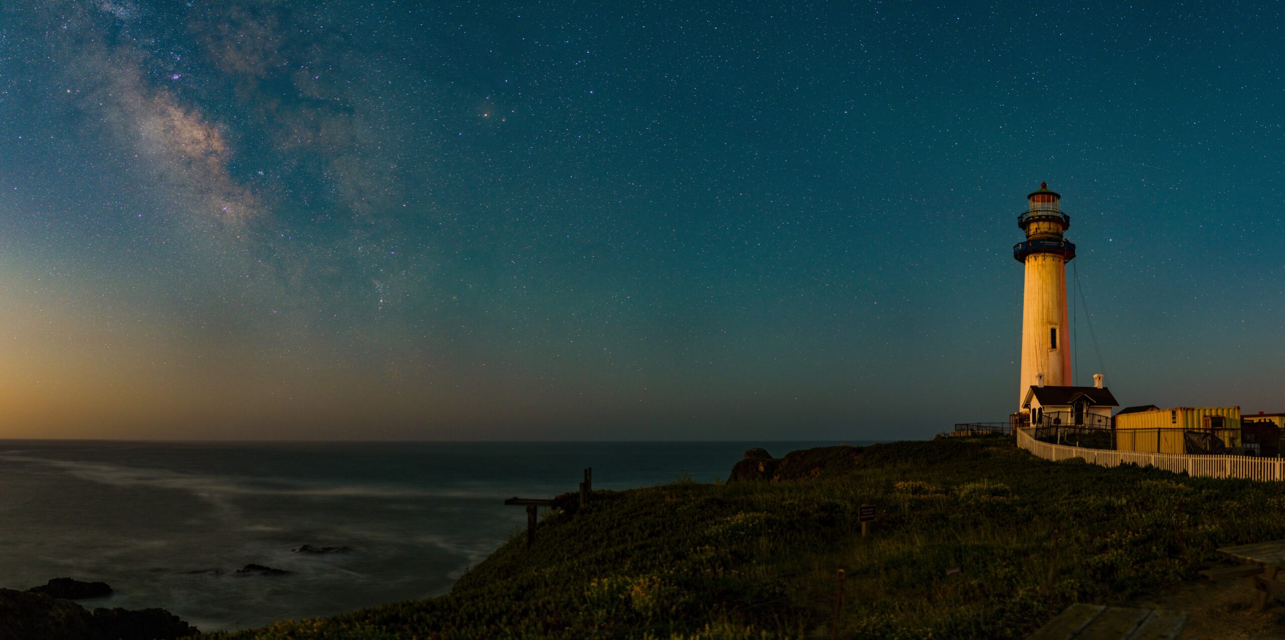
On the first night, I went to Pigeon Point Lighthouse and stayed at the hostel. This is a great spot to visit even if you don’t care for astronomy! It is much closer than Big Sur or Point Arena, but still has that “Highway 1” aura, along with great sunsets and views of birds and sea lions.
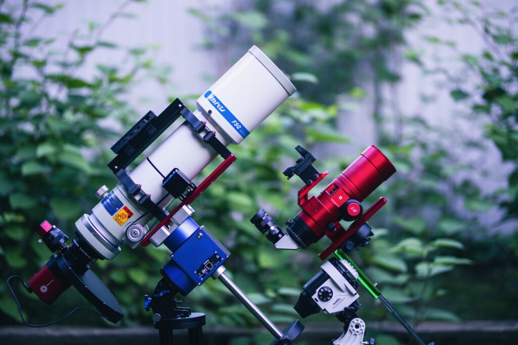
To get a wider field of view, I used the 250mm RedCat 51 telescope. Here is a picture of the RedCat next to its big brother the FSQ. Both are f/5 scopes, meaning that the shorter focal length makes the RedCat 2x smaller, and a lot lighter to carry!
I had technical issues on the first night, so I stayed a second and got a good 4 hours of imaging data, mostly with the L, B, and G filters, since the target went behind a building before collecting much R data. So the picture was incomplete, but the views of the lighthouse were nice after the moonrise.
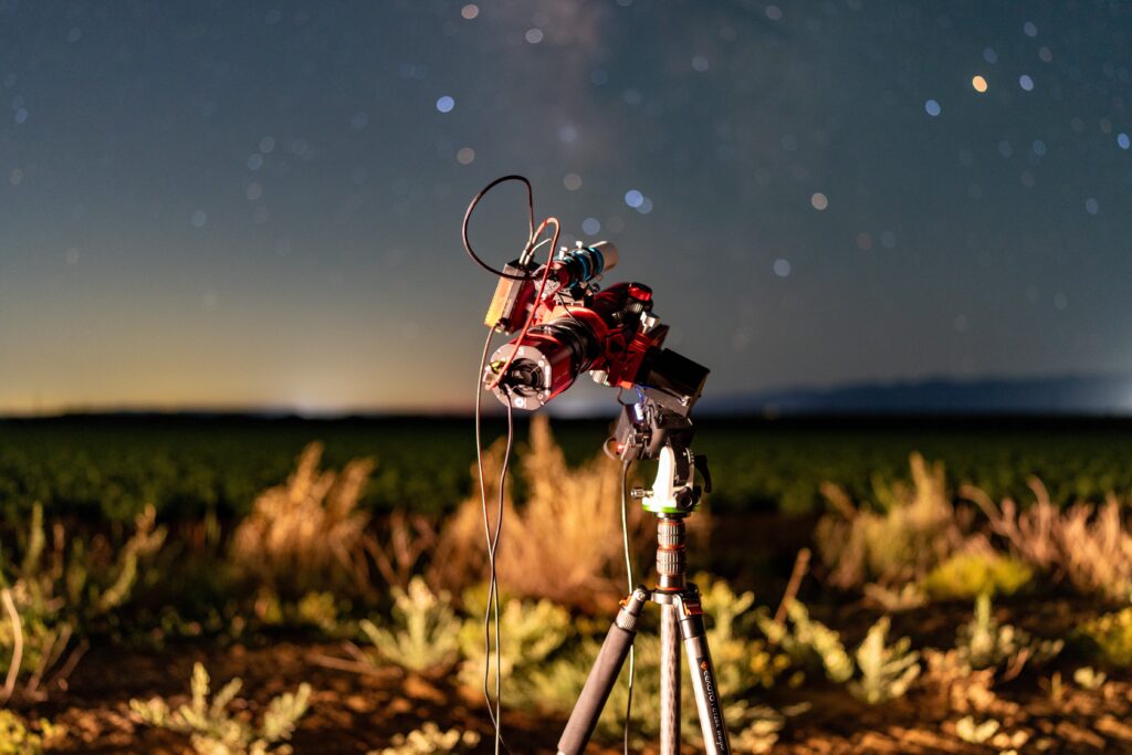
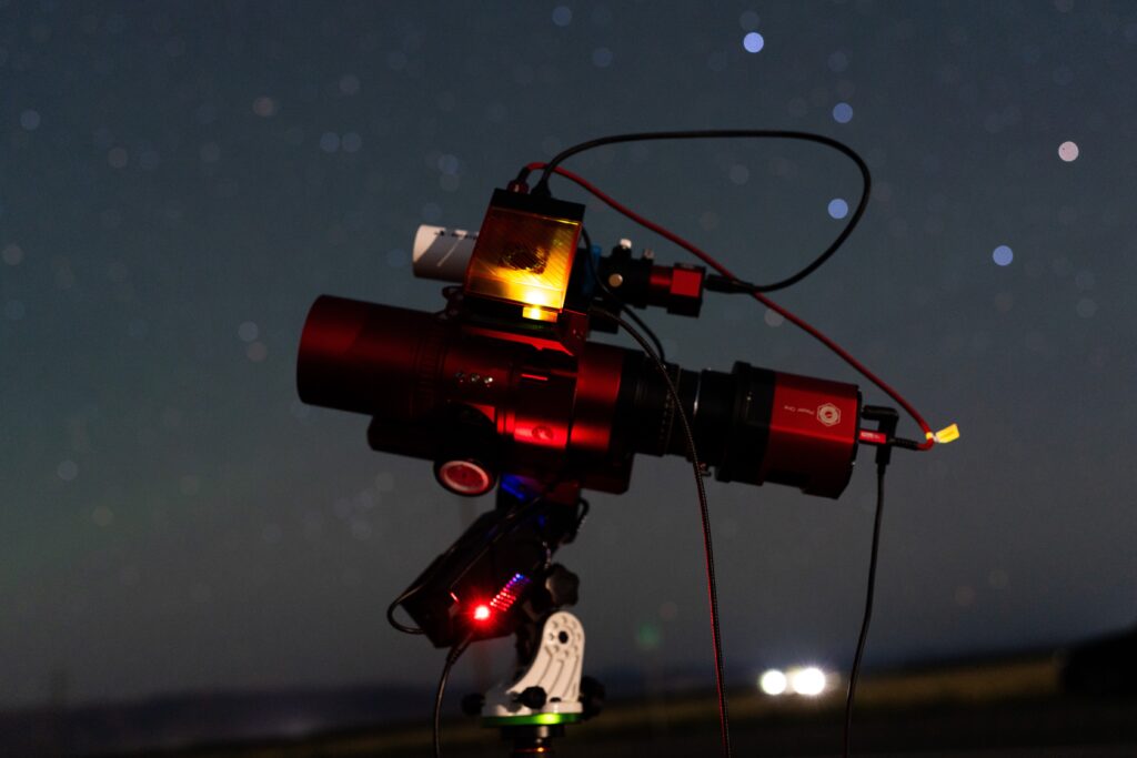
To fill in the missing data, I went out the next weekend. This time, I drove north to Williams, a small farming town on I-5 between Sacramento and Redding. You can get to reasonably dark inland sites by heading north on I-80, turning left on I-505 and later I-5, which passes by the towns of Winters, Williams, and Willows (don’t conduse the names!), and lots of farmland. It over 100º that afternoon, but I arrived well after sunset and the temperature was dropping fast. I set up the RedCat by CA-20 and took data all night, sleeping between filter changes, which I had to do manually because the filter wheel overloads this tiny mount. Here are two shots of the telescope. The first is illuminated by passing headlights. There were a lot of cars on that road, even well into the night.
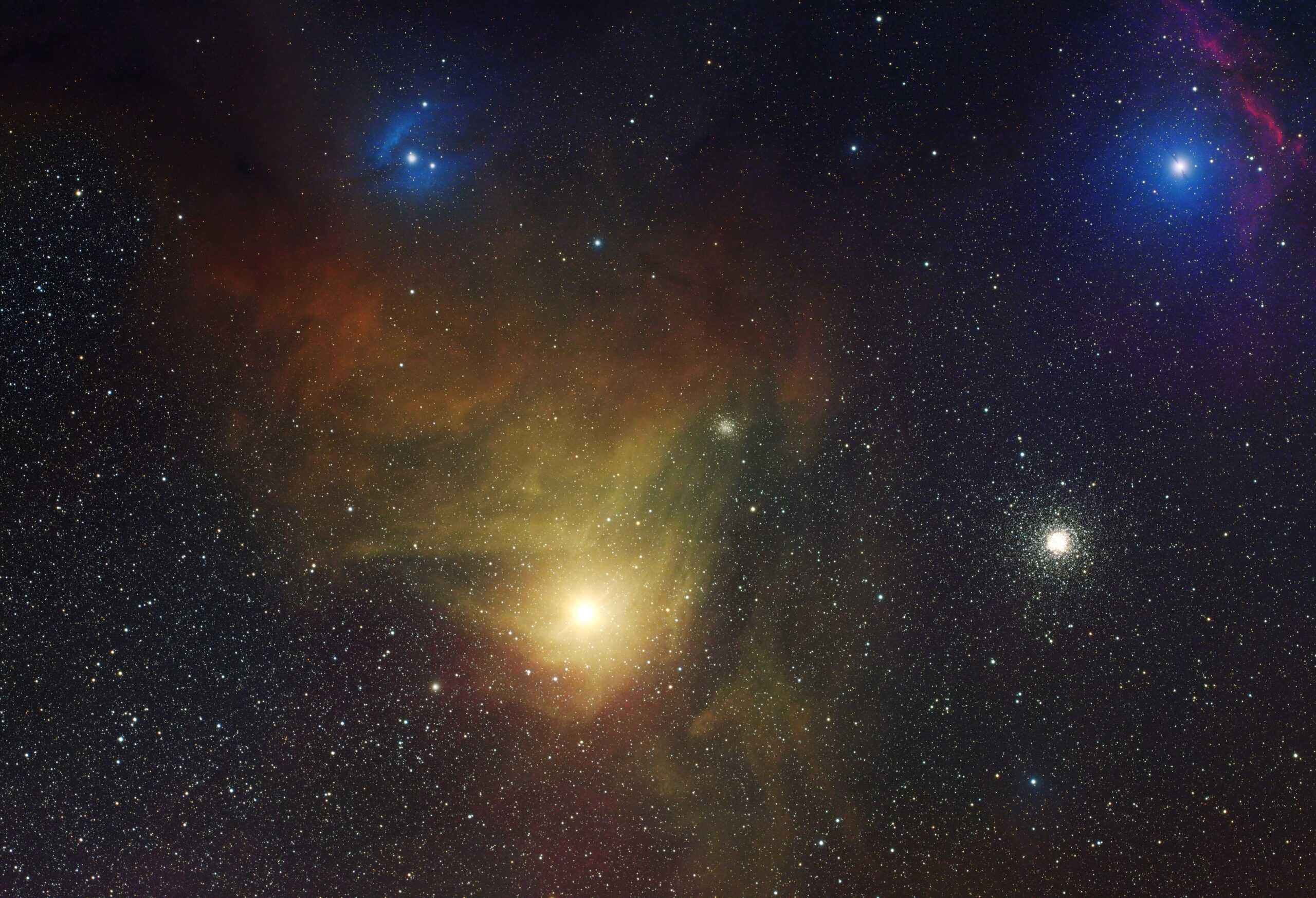
This gave me enough data to complete the image. Now, finally, I could frame Antares at that “just-right” focal length of 250mm!
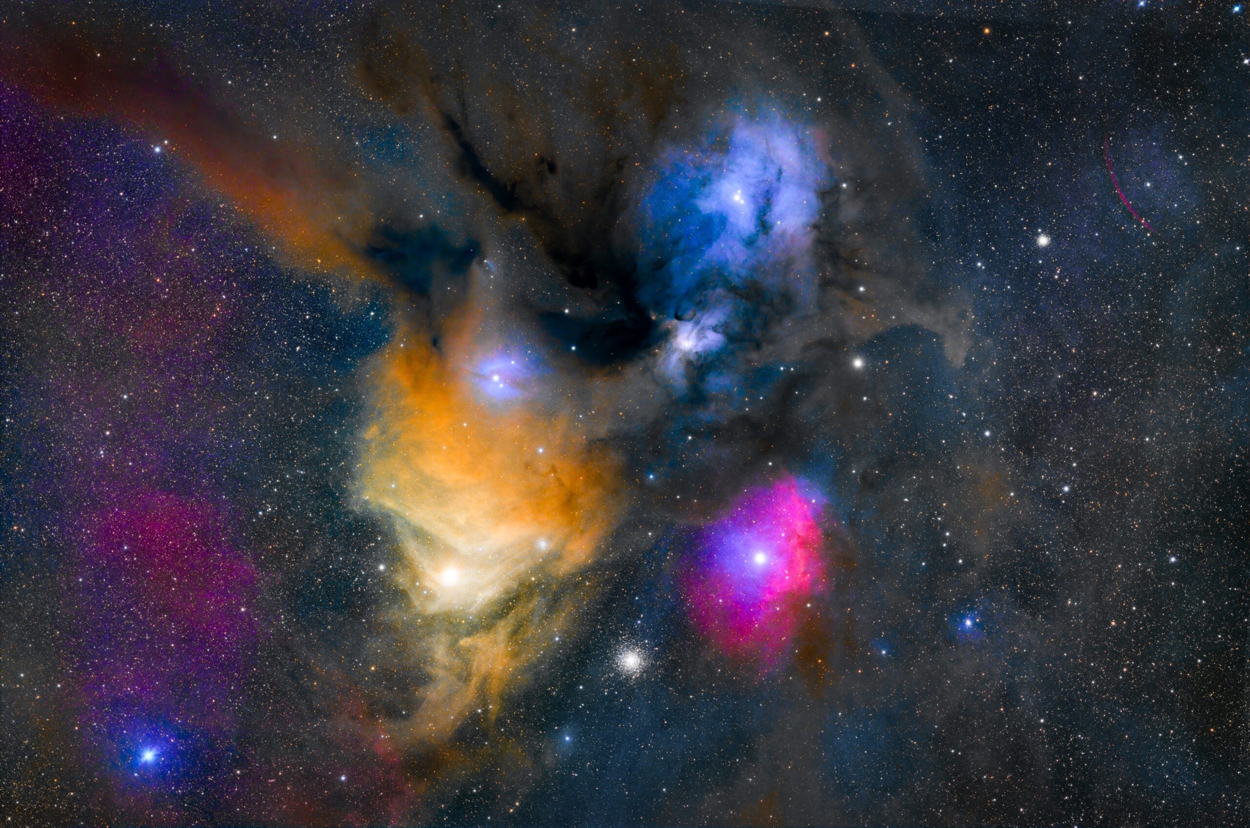
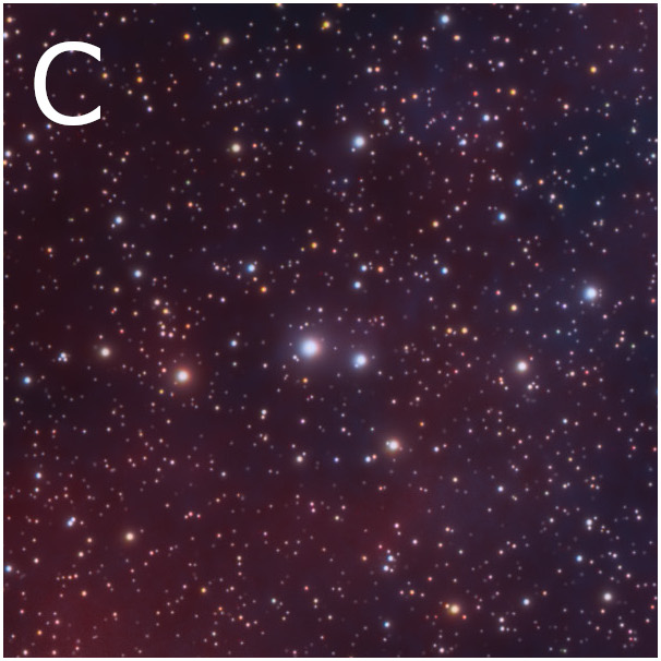
This photo brings out all the parts of that unique object — the yellow dust near Antares, red H-alpha near Alniyak, the blue reflection near ρ Ophiuchi, the tight Crab globular cluster, and the gray-black “dark nebulae” — un-illuminated dust in the foreground that casts shadows over the scene.
Processing Trick: Post-Sharpening Alignment
This section’s for nerds only, and it addresses a common problem of ugly multi-colored stars that appear when postprocessing astro images. I have observed this problem before, but only recently, when editing the Antares image, did I find the fix.
The problem arises from lens aberrations and the way that we fix them. All lenses are imperfect and have optical aberrations. These aberrations lead to a “blurring” of the image according to some point-spread function (PSF). Each lens aberration — coma, astigmatism, spherical aberration to name a few — gives rise to its own PSF, and the total aberration is the combination of them all. Aberrations are stronger in the corners, which is why corner stars tend to look ugly and elongated. Daytime photographers notice the same thing. Even on premium lenses, the corners of an image at maximum aperture always look a little “soft”.
Since aberrations cause blurring, which is a simple mathematical convolution, we can correct for them using a technique called “deconvolution”. Once the PSF is known, we can “invert” the convolution and recover the original image. But this is challenging because deconvolution adds noise (a convolution is a filter in Fourier space, and its inverse needs to re-amplify the high-frequency components that were filtered out). So deconvolution requires a very low-noise image to be effective, as well as good statistical modeling obtain the PSF and noise model. Modern tools like BlurXTerminator (BXT) use AI to assist with this step, inferring the PSF by fitting tens of thousands of stars, and estimating the noise to determine how much sharpening is possible.
Below, I apply BXT to the corners of my image (luminance master). Look at how it cleans up those stars!
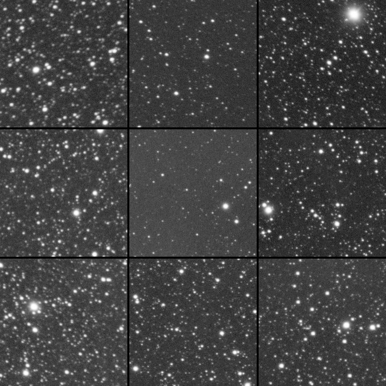
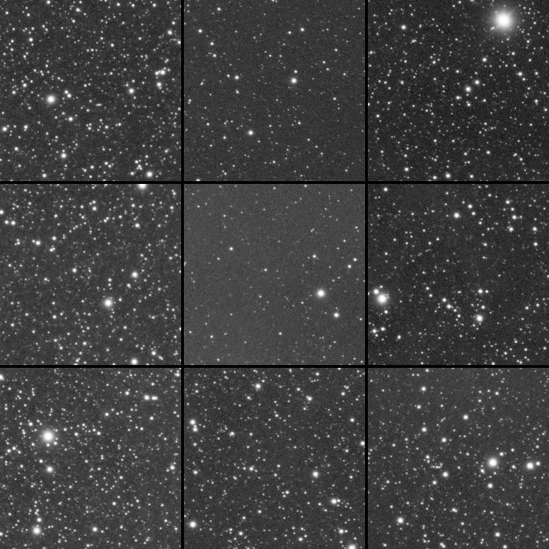
But when we apply deconvolution, we quickly run into problems from chromatic aberration, where the telescope focuses different colors to slightly different spots. This is reported in a telescope’s spot diagram. William Optics and Takahashi make high-quality products and proudly post the spot diagrams on their website. Here is the one for the RedCat 51.
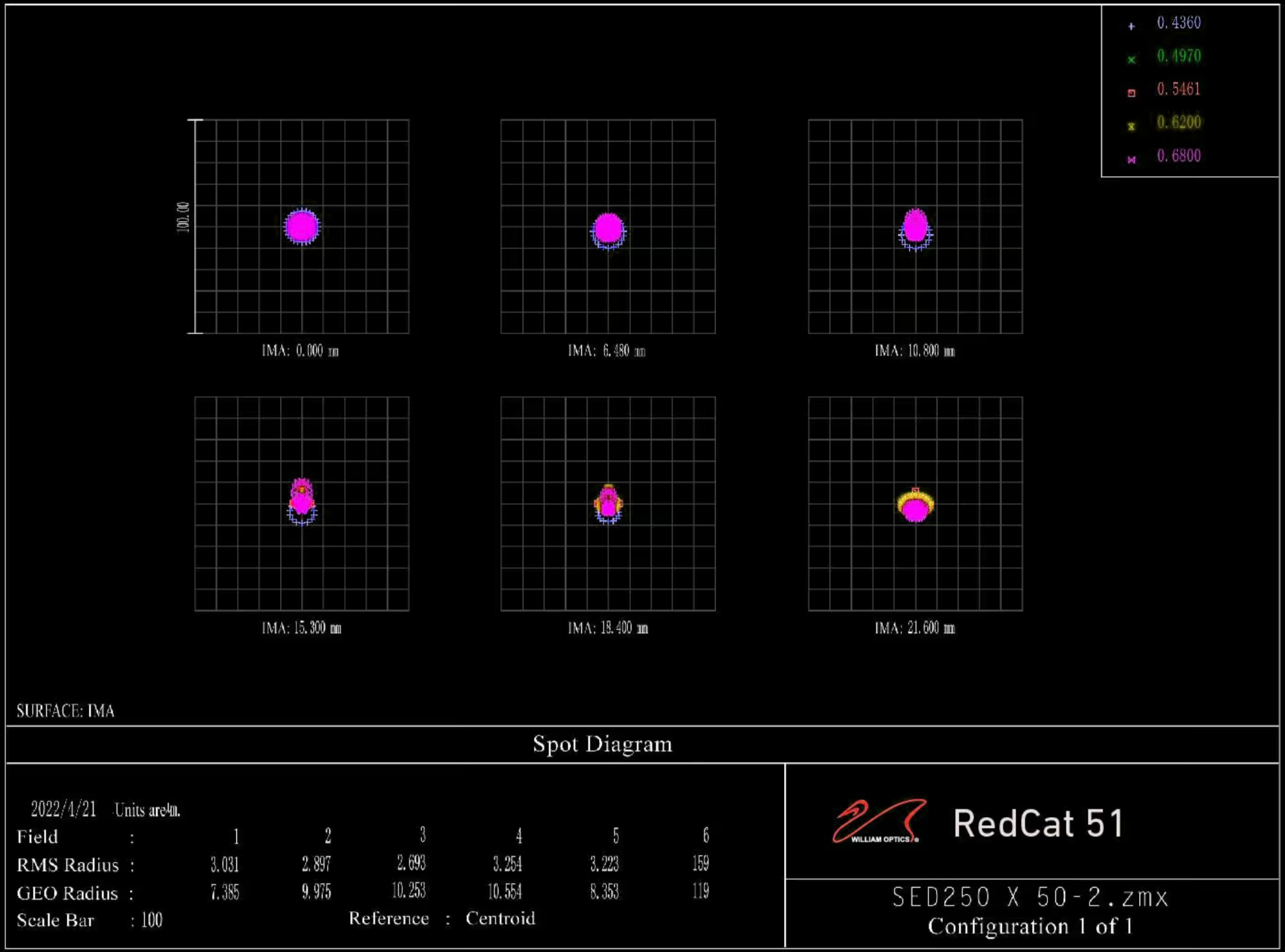
Now let’s apply deconvolution, independently, for all three colors. The spot sizes shrink, but the spacing between the red, green, and blue centroids remains the same. So relative to the spot size, the aberration is now bigger!
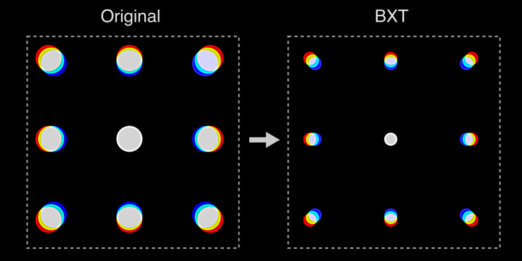
This makes chromatic aberration much more visible, especially after you apply a saturation curve to bring out the color of the stars. Below I give an example from the Crescent Nebula image that I shot back in this post. Notice how some of the bright stars have a halo that is red on one side, and blue on the other.
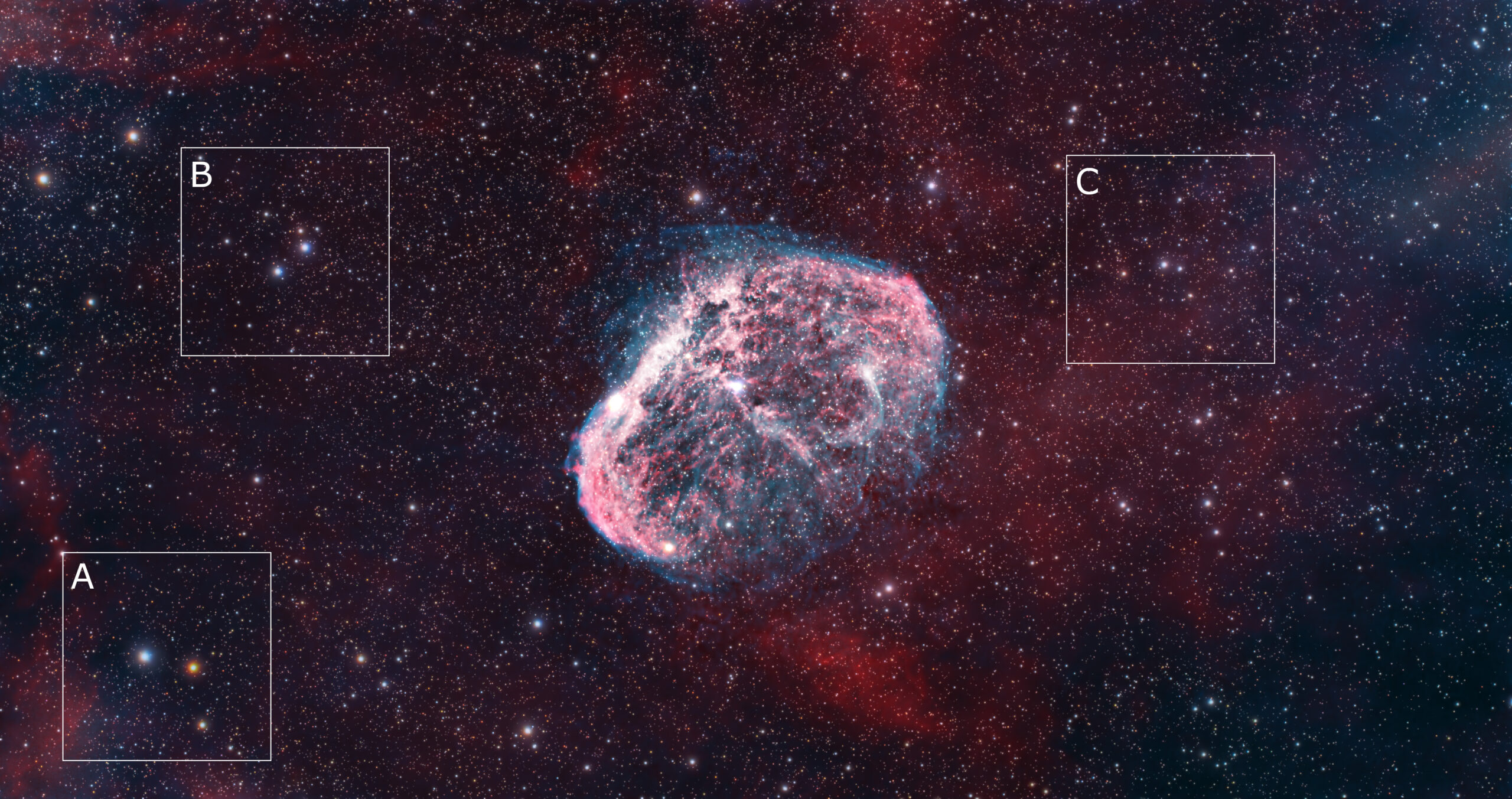
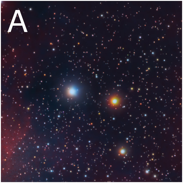
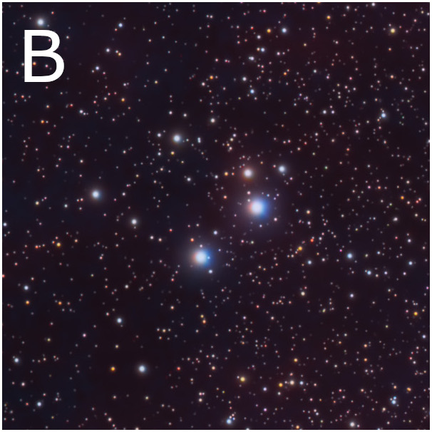
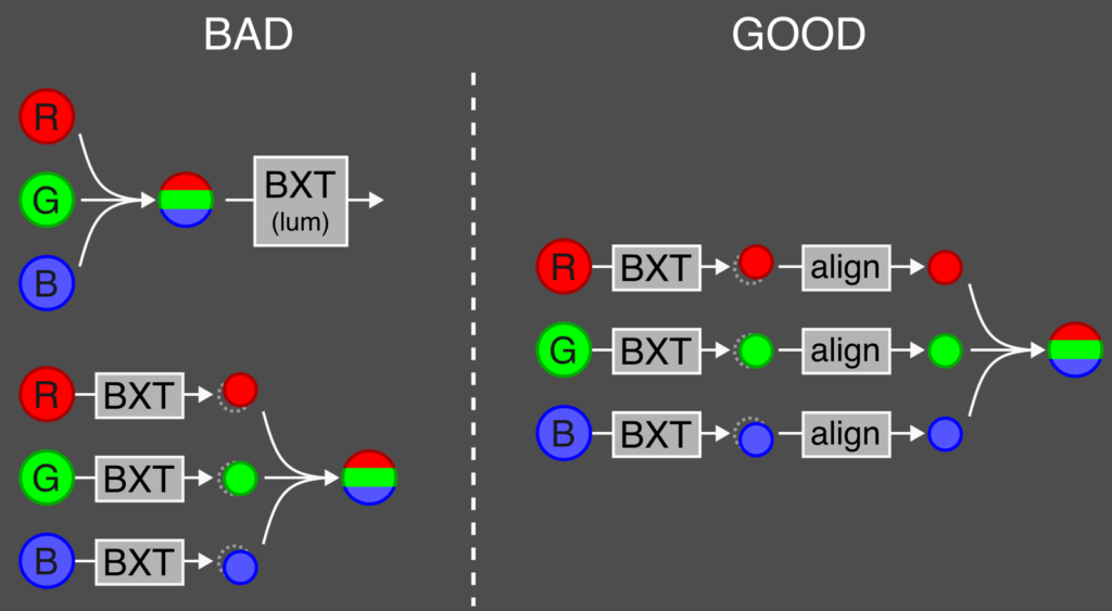
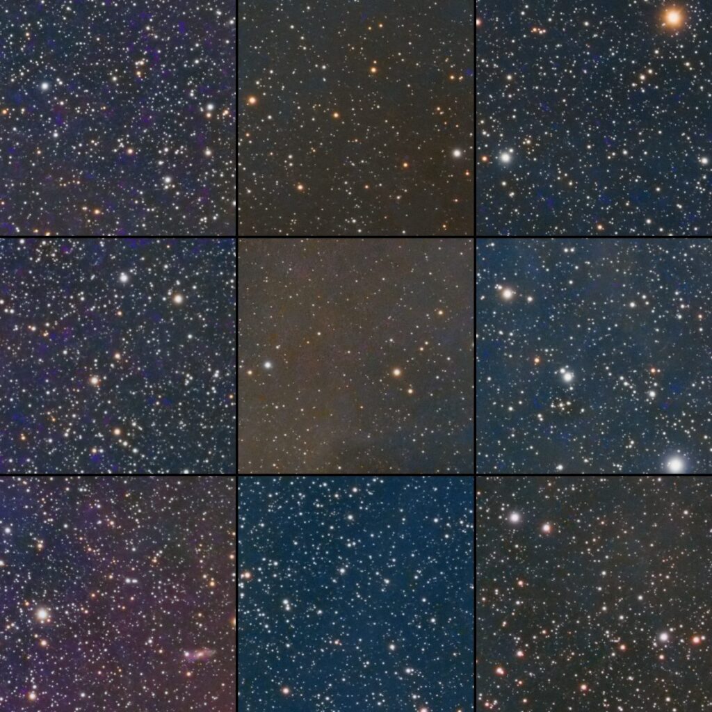
While processing Antares, I developed a simple trick: post-sharpening alignment. After applying BXT to each frame separately, I use a tool like StarAlignment to align it a master frame (for this I use the luminance, since it has the cleanest signal). This is in comparison to previous approaches I’d used: either to deconvolve the RGB color image, or to deconvolve the separate colors and then combine into an RGB image. The alignment step lets us correct for any (lateral) chromatic aberration, giving clean, monocolor stars.
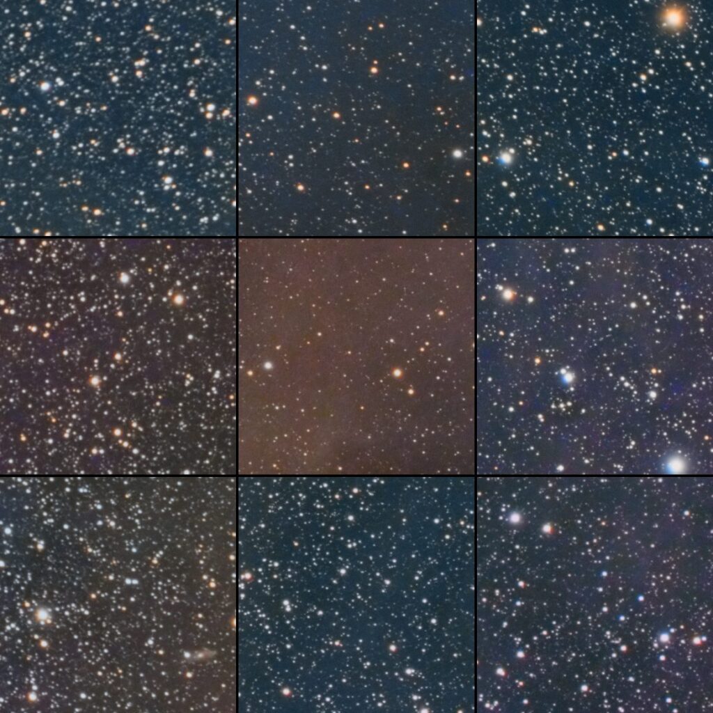
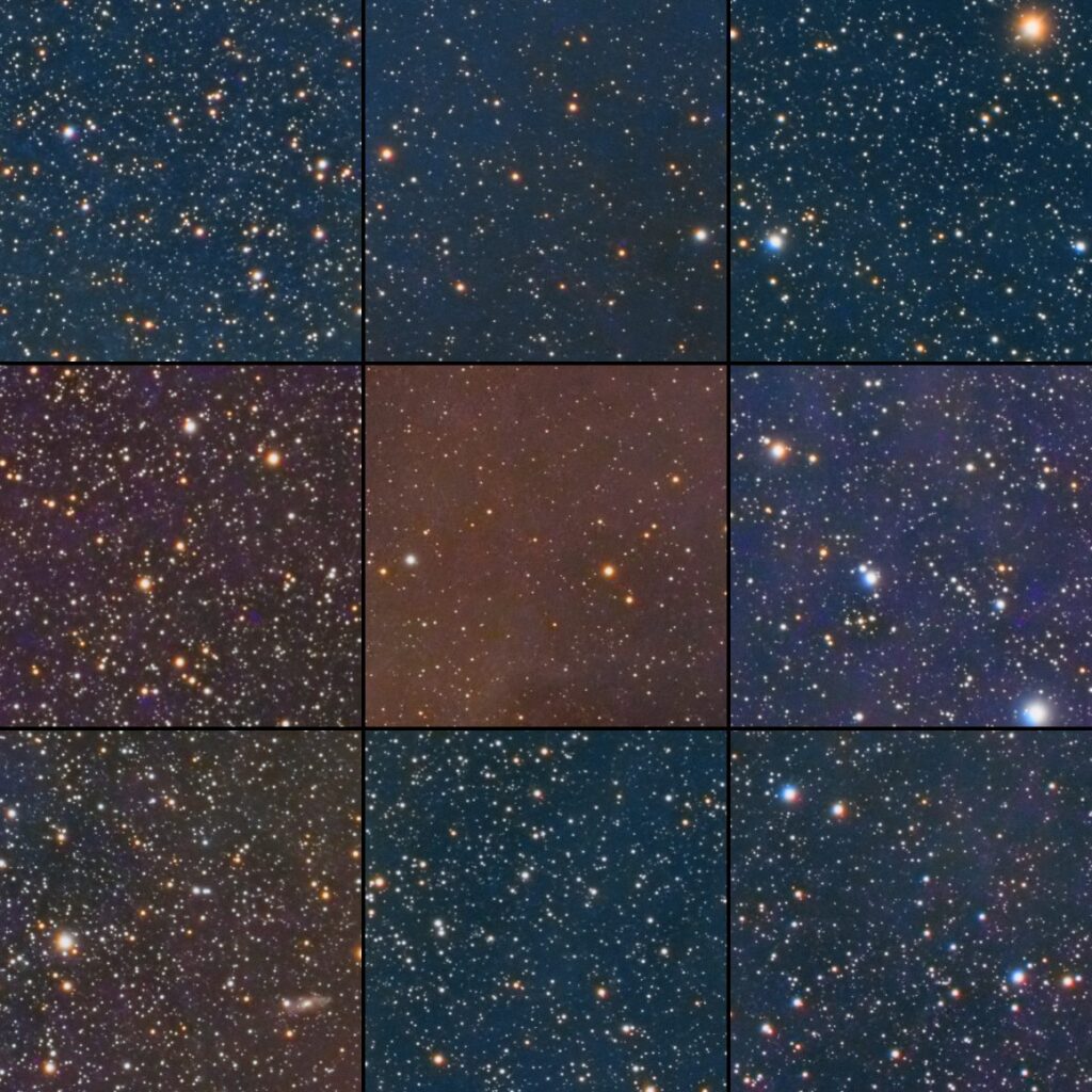
Below, I show corner aberrations for my Antares shot, where all postprocessing steps are identical except for the deconvolution. Three cases are presented:
- No correction
- BXT
- BXT + post-sharpening alignment
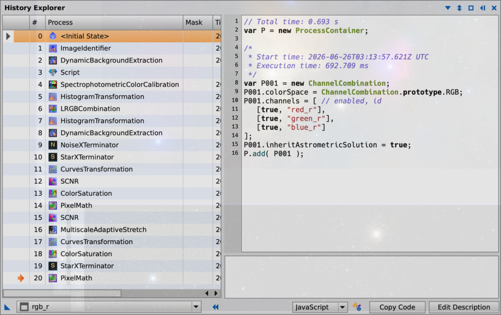
Besides the alignment trick, I didn’t do anything unconventional when editing this image. Just a few steps of background subtraction, a histogram stretch, LRGB combination, more background extraction (the gradients were annoying), SCNR to remove a weird green glow, curves and color saturation, and star removal to facilitate separate star processing. Here’s the whole process flow if you want to try 🙂